Monobot
Monocular robot using AprilTag EKF for pose estimation
Code: monobot
Overview
Monobot is a differential-drive robot with a monocular camera that utilizes an extended Kalman filter (EKF) for pose estimation. AprilTag fiducial markers of known sizes are placed around the environment and detected by Monobot’s camera. As the robot drives around the environment the AprilTag 3 algorithm [1] estimates the pose of the markers in the camera frame, and provides this pose as a measurement to the EKF. The EKF then estimates the Monobot pose and AprilTag marker positions in the world frame.
Hardware
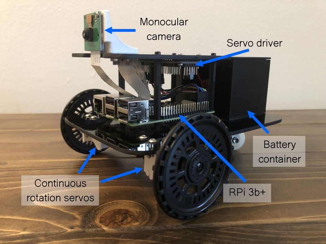
Monobot consists of two continuous rotation servo motors, a Raspberry Pi (RPi) 3 model B+ running an Ubuntu 20.04 server, a 16 channel 12-bit PWM servo driver and a RPi camera module 2. Components are attached to black acrylic sheets, and the servos are attached using 3D-printed mounts. The robot body was designed in OnShape.

Experiment
To verify the implemented EKF method (kalman_filter.py), six AprilTag markers were placed in the environment. Monobot was remotely controlled to drive in a loop at a constant speed. The locations of the markers were measured with a measuring tape to provide an initial estimate for the marker positions.
To visualize the trajectory and AprilTag detections in real-time during the experiment, trajectory and image data is streamed over the wifi network from the RPi. A custom solution was developed using Flask (Python web framework) in combination with Plotly.js (JavaScript graphing lib). The result is shown in the following video.
Extended Kalman Filter
This section is limited to describing the process dynamics and measurement model used for the implemented EKF. For further explanation of the EKF method, [2] provides a nice introduction.
Notation
Four coordinate frames are used throughout this section: the world coordinate frame, \(W\), the robot body coordinate frame, \(B\), the camera coordinate frame, \(C\), and the \(i\)-th AprilTag marker coordinate frame, \(M_i\). In this context a term of the form \(x_B^C\), for example, denotes the \(x\)-position of the body frame origin expressed in the camera frame. To simplify notation, when terms are expressed in the world frame the \(W\) superscript is often dropped when context is clear (e.g. \(y_B^{} := y_B^W\)).
Process Dynamics
The process dynamics are continuous and nonlinear:
\[\dot{\mathbf{x}} = f(\mathbf{x}, \mathbf{u}, \mathbf{w}) = \begin{bmatrix} \dot x_{B}^{} \\ \dot y_{B}^{} \\ \dot \psi_{B}^{} \\ \dot x_{M_1}^{} \\ \dot y_{M_1}^{} \\ \vdots \\ \dot x_{M_n}^{} \\ \dot y_{M_n}^{} \end{bmatrix} = \begin{bmatrix} v_{B}^{}\cos(\psi_{B}^{}) \\[1.45pt] v_{B}^{}\sin(\psi_{B}^{}) \\[1.45pt] \omega_{B}^{} \\[1.45pt] 0 \\[1.45pt] 0 \\[1.45pt] \vdots \\[1.45pt] 0 \\[1.45pt] 0 \end{bmatrix} + \mathbf{w},\quad \mathbf{u} = \begin{bmatrix} v_{B}^{} \\ \omega_{B}^{} \end{bmatrix},\]where \((x_{B}^{},\,y_{B}^{})\) is robot position, \(\psi_{B}^{}\) is robot heading angle, and the control inputs \(v_{B}^{}\) and \(\omega_{B}^{}\) are speed and turn rate, respectively. The position of the \(i\)-th AprilTag marker is denoted by \((x_{M_i}^{},\,y_{M_i}^{})\), and the process noise vector is \(\mathbf{w}\). Note \(n+1\) markers are placed in the environment, where the first marker defines the origin such that \((x_{M_0}^{},\,y_{M_0}^{}):=(0,\,0)\).
To perform state prediction, a fourth-order Runge-Kutta integration scheme (RK4) is used. To discretize the continuous-time process dynamics (for use in computing the predicted covariance matrix), a first-order Taylor expansion is used.
Measurement Model
The EKF measurement step is performed when one or more fiducial markers are viewed by the camera. A measurement of the \(i\)-th AprilTag marker can be described as follows:
\[\mathbf{z}_{M_i}^{} = \begin{bmatrix} x_{M_i}^B \\ y_{M_i}^B \\ \psi_{M_i}^B \end{bmatrix} + \mathbf{v}_{M_i}^{},\]where \(\mathbf{v}_{M_i}^{}\) is the measurement noise for the \(i\)-th marker. Note the AprilTag algorithm outputs the pose of frame \(M_i\) with respect to frame \(C\). However since the transformation from frame \(C\) to frame \(B\) is constant, we can use the above expression of \(\mathbf{z}_{M_i}^{}\) as the measurement to allow for a simpler measurement model.
To determine the measurement model \(h_{M_i}^{}(\mathbf{x}, \mathbf{v}_{M_i}^{})\) for observed marker \(i\), we need to express \(\mathbf{z}_{M_i}^{}\) in terms of \(\mathbf{x}:\)
\[\begin{align*} \begin{bmatrix} x_{M_i}^B \\ y_{M_i}^B\end{bmatrix} &= R_W^B \left(\begin{bmatrix} x_{M_i}^W \\ y_{M_i}^W\end{bmatrix} - \begin{bmatrix} x_B^W \\ y_B^W\end{bmatrix}\right)\\ &= \begin{bmatrix} \cos(\psi_B^{}) & \sin(\psi_B^{}) \\ -\sin(\psi_B^{}) & \cos(\psi_B^{}) \end{bmatrix} \begin{bmatrix} x_{M_i}^{} - x_B^{} \\ y_{M_i}^{} - y_B^{} \end{bmatrix}\\ \end{align*}\] \[\mathbf{z}_{M_i}^{} = \boxed{h_{M_i}^{}(\mathbf{x}, \mathbf{v}_{M_i}^{}) = \begin{bmatrix} (x_{M_i}^{} - x_{B}^{})\cos(\psi_{B}^{}) + (y_{M_i}^{} - y_{B}^{})\sin(\psi_{B}^{}) \\ (y_{M_i}^{} - y_{B}^{})\cos(\psi_{B}^{}) - (x_{M_i}^{} - x_{B}^{})\sin(\psi_{B}^{}) \\ \psi_{M_i}^{} - \psi_{B}^{} \end{bmatrix} + \mathbf{v}_{M_i}^{}},\]where \(\psi_{M_i}^{}\) is a known constant. The full measurement model is created by vertically stacking the individual measurement model vectors for each visible AprilTag marker. For example if markers 0 and 2 are visible, the full measurement model is \(h = [h_{M_0}^T\; h_{M_2}^T]^T\), where arguments are dropped to simplify notation.
Future Directions
- Control Input Bias: To improve EKF estimation accuracy, it is desirable to estimate how much the control inputs deviate from ground truth values (i.e. control input bias). For example the commanded speed may be 1 m/s, but the ground truth speed may be 1.2 m/s. Control input bias was initially part of the EKF state vector, and was made observable by artificially extending the measurement of the \(i\)-th marker to include \([\dot x_{M_i}^B\;\; \dot y_{M_i}^B\;\; \dot \psi_{M_i}^B]^T\). This method provided poor control input bias estimation, likely due to sparse AprilTag detections. As such, a future direction includes fusing measurements from a high-rate sensor such as an IMU.
- Trajectory Tracking: The current EKF implementation was verified using human teleoperation (EKF_teleop.py). However, a trajectory tracking method using dynamic feedback linearization (from [3]) was implemented (EKF_autopilot.py), but needs some debugging.
References
[1] M. Krogius, A. Haggenmiller and E. Olson, “Flexible Layouts for Fiducial Tags,” 2019 IEEE/RSJ International Conference on Intelligent Robots and Systems
[2] G. Welch and G. Bishop, “An Introduction to the Kalman Filter,” 2006
[3] A. De Luca, G. Oriolo and M. Vendittelli, “Control of Wheeled Mobile Robots: An Experimental Overview,” 2001 Lecture Notes in Control and Information Sciences